Video: Scattering I
Slides
In the previous two chapters we have focused our attention on situations where a particle is bound inside a potential well. This is a situation which is very prevalent and important. In these cases, we saw that a particle can only have special discrete energies.
Prior to this we studied a free particle — when there were no forces acting, and so far this has been the only instance of a non-bound state that we have considered. In this final chapter considering quantum mechanics in 1D, we will now return to a situation where a particle is non-bound, but one that is more interesting and physical than the free particle.
We will consider the situation where a particle scatters off of a target, which we model by a change in potential. This is a very important physical situation which arises in a wide range of situations, from neutrons scattering in condensed matter physics, to the scattering of particles off each other in particle detectors. Our goal here is to understand the basics of scattering in quantum mechanics.
We will consider just one simple potential — an abrupt change. The motivation for studying this is somewhat similar to our motivation for studying the infinite square well. While this is far from realistic, it is simple enough that we can solve exactly for the energy eigenstates (which are now no longer momentum eigenstates, like for the free particle). We can then use these to numerically study what happens when a wavepacket scatters off of the step.
We will uncover one final new aspect of quantum mechanics, which is almost the complete opposite of tunnelling. Whereas in tunnelling a quantum particle enters a region of space it should not have enough energy to enter, in this chapter we will see that quantum particles reflect off of abrupt changes in potential — whether those changes are positive or negative. That is, quantum particle reflect off of cliff edges, and therefore fail to enter a region that they would definitely enter.
9.1The finite step potential
In this chapter we will consider the following potential function
depicted in Figure 9.1.

Figure 9.1:The potential step. The potential energy vanishes for , and is equal to for . In the figure we have taken , although in the mathematics that follows, we make consider to be either positive or negative.
This corresponds to an abrupt change in potential from to at the origin. It is important to note that could be either positive or negative, meaning that the potential energy either steps up or down. We will primarily keep in the back of our mind that , but will also discuss what happens if .
Our goal, as always, is to find the energy eigenstates of the potential well, which we will do by solving the TISE to find the energy eigenfunctions. Since the particle isn’t bound, we expect that the energy should vary continuously and the eigenfunctions shouldn’t be physical and normalisable. We will indeed see that this is the case below.
9.2Energy eigenfunctions of the potential step
The approach that we will take is going to be similar to the infinite square well — since the potential energy is specified in pieces, we will seek to solve for the energy eigenfunctions in pieces also. We will call the region to the left of the step region I () and the region to the right of the step region II (). We will call the energy eigenfunctions in these regions and respectively, such that
After solving for the two pieces, we will join them together using the continuity of energy eigenfunctions, as we did in the case of the eigenfunctions of the infinite square well (with one additional new ingredient).
9.2.1Energy eigenfunctions in Region I
We will start off considering Region I, to the left of the step. In this region . Therefore, just as happened inside the infinite square well in Section 7.2.2,
and so, just as we were able to do there, we can immediately write down the energy eigenfunction, as this is the same Hamiltonian (and the same as the free particle also!). As we discussed in Section 7.2.2, any function of the form
will be an eigenfunction, where and are arbitrary complex numbers, where the corresponding energy eigenvalue is
Just as in the case of the infinite square well, we don’t yet know which superposition of and we should take (i.e. how to choose and ). For the moment we will leave them general, and see that we can determine them later, using continuity.
9.2.2Energy eigenfunctions in Region II
We now turn our attention to Region II, to the right of the step. In this region . In this region , and the TISE we want to solve is
We can move the term involving from the left-hand to the right-hand side, to express this as
Since is just a constant, this has again exactly the same form as for a free particle except we are looking for an eigenvalue of , instead of . The only subtlety we need to be careful about is that previously we tacitly had . We will therefore make the same assumption that , i.e that . Physically this means we are going to consider situations where the particle has enough energy to classically climb the potential step. We will study the opposite situation as an exercise.
Given the above, we can once again write down the solution! In particular, the energy eigenfunction in region II will be identical in form to an energy eigenfunction without a potential and with energy . The solution is therefore
where and are two new constants (that we will also need to determine in due course), and
Taking a step back (no pun intended), this makes perfect sense. Once the particle has passed the step, its potential energy has increased by . The total energy is still , and so the kinetic energy of the particle is now . This is why we see that energy eigenfunction has exactly the same form as an energy eigenfunction with .
9.2.3Right-moving and Left-moving eigenstates
Putting everything together that we have learnt so far, we know that the energy eigenfunctions of the potential step have the form
where , , and are complex constants, that we need to determine, and and are functions of the energy and step height, specified via (9.5) and (9.9) respectively.
In order to make progress, we first need to cast our mind back to Chapter 6: Free particle, and the fact that we found there two degenerate eigenstates for each energy. What were the two degenerate eigenstates? They were the two momentum eigenstates with equal and opposite momentum, and .
Here we are going to have something very similar. What we need to understand is what are the analogue of these two eigenstates here? The key insight is that a momentum eigenstate with positive momentum represents a particle moving to the right, while an eigenstate of negative momentum represents one moving to the left. We thus want to identify right-moving and left-moving eigenstates of the step, as the two basic states of interest.
We will be able to do this, but we need to use a bit of foresight. In particular, as stated in the introduction, quantum particles reflect off of abrupt changes in potential, irrespective of whether that is a positive or negative change. What does this imply about left-moving and right-moving states? Let us start off by considering a right-moving state in region I, which would correspond to (since this has the same form as a positive momentum state in this region, if ). When it reaches the step, it will reflect, creating a component (essentially a negative momentum state), and also pass through, creating a component in region II (with positive momentum). In region II however, there will be no negative momentum component (i.e. component of the form ).
This is summarised graphically in Figure 9.2 (a).

Figure 9.2:Right-moving and Left-moving situations. (a) In a ‘right-moving’ situation, a particle approaches the step from the left, with positive momentum. It is then partially reflected by the step, and partially transmitted. (b) In a ‘left-moving’ situation, everything is reversed. The particle approaches the step from the right with negative momentum. It is then partially reflected, and partially transmitted.
This line of reasoning suggests that we should take in (9.10) when considering right-moving eigenfunctions. We will denote this eigenfunction by (‘R’ for ‘right-moving’), and their general form will be
A similar line of reasoning, which you are encouraged to think through, and which is summarised in Figure 9.2 (b), suggests that we should take in order to define left-moving eigenfunctions, which we denote by , and have the general form
(where we now use primes on the constants , and , to highlight the fact that this is a distinct eigenfunction with distinct unknown parameters at this stage).
In what follows, we will focus on right-moving particles, and leave the corresponding analysis of left-moving particles as an exercise.
9.2.4Continuity of eigenfunctions and their first derivatives
Video: Scattering II
Slides
We will now see how we can fix the unknown constants in the eigenfunctions. First, as we learnt in Section 7.2.3, energy eigenfunctions must be continuous. We must apply this fact at the potential step (), as for general choices of , and this won’t be the case. In particular, from (9.11) we see that at (since we include in region II). If we approach the origin from region I, i.e. take from below, we find . In order for eigenfunction to be continuous, we must therefore have
We can use this equation to solve for one of the constants, e.g. to eliminate directly. This still leaves us with two constants.
To fix another constant, we need to introduce one further fact about energy eigenfunctions:
The first spatial derivatives of energy eigenfunctions are also continuous.
Like many good rules, this one has an exception! There is only one situation where the spatial derivative of an energy eigenfunction doesn’t have to be continuous, and this is precisely the situation we encountered when studying the infinite square well: it is when the potential is infinite.
We therefore didn’t introduce this fact previously, as we happened to be in the one exceptional case. We are introducing now as for the potential step, the potential is finite everywhere and hence we do need to impose continuity of the spatial derivative.
What does it mean for a function to have a continuous derivative? This means that there will be no kinks in the graph — no points where the function changes slope abruptly. Thus energy eigenfunctions cannot have jumps or kinks (except where the potential is infinite).
Let us now see how to apply this. We can easily calculate the spatial derivative in the two regions, to find that
(where we have substituted already). We then demand continuity just as did above. At , we have . On the other hand, if we approach 0 in region II from below, we find on Thus, in order to have a continuous first spatial derivative, we must have
We can use this to solve for , which after a small amount of re-arranging, leads to
What about the final constant ? As always, this is in fact just an overall normalisation constant. Since here we are considering a non-bound state, energy varies continuously, and energy eigenfunctions are unnormalisable. We can therefore take for simplicity. There is no real natural choice for , and this is as good as any. Altogether, we therefore find that the energy eigenfunction of energy for a right-moving particle is
This eigenfunction (for one choice of ) is depicted below in Figure 9.3.
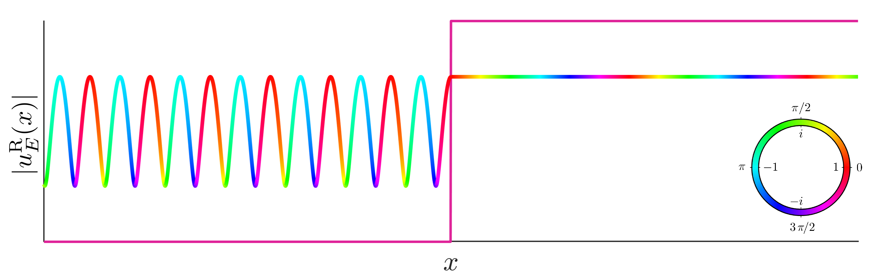
Figure 9.3:Right-moving energy eigenfunction of the potential step. Colour plot of a right-moving energy eigenfunction, given in (9.17). For illustrative purposes, we also plot the potential step, to highlight where it is in relation to the wavefunction (the height of the step has relation to the amplitude of the wavefunction). On the left of the step, where there is both the incoming and reflected component of the wavefunction, there is interference, leading to sinusoidal oscillations. On the right, where there is only the transmitted component, the modulus of the wavefunction is constant.
As a summary of what we have achieved: in (9.17) we have found the wavefunction of the quantum step Hamiltonian with constant energy , that is ‘right-moving’, in the sense that when we look on the left of the step, we only have a positive momentum component. We found this by using two key mathematical properties of energy eigenfunctions: that they are continuous (as previously seen), and that they have a continuous derivative (which is new here). More informally, this ensured that the function has no ‘jumps’ and no ‘kinks’. Just as with the free particle, there is a second degenerate energy eigenfunction of energy . This corresponds to a left-moving particle, and you will solve for it as an exercise below.
We will now analyse some of the interesting physics of these eigenfunctions, before briefly outlining how they can be used to study the dynamics of particles (although you won’t be expected to do this yourself, only to appreciate qualitatively what is found).
9.3Reflection and transmission coefficients
What we would like to understand now as quantitatively as possible, is the meaning of the superposition appearing in (9.17). We will see how to do this in terms of so-called reflection and transmission coefficients.
The main point we would like to understand is the significance of (9.16), namely how the amplitude of the reflected component relates to the amplitude of the incoming component (which we have taken to be for simplicity).
We can start by considering an extreme case: that if no potential step. That is, we can set , and ask what happens to the energy eigenfunction. In this case, we know what we should hope to find, since this corresponds to a Chapter 6: Free particle, and hence the energy eigenfunctions should just be momentum eigenfunctions. This is precisely what we find, since from (9.9), in this case , and hence , leaving us with simply the component for all , corresponding to a momentum eigenfunction with momentum .
This is reassuring, but what about for ? Here we see that depends upon the energy relative to the step height, since and specify and . This shows that the reflected component is energy dependent.
The way this is usually studied is by introducing the so-called reflection coefficient: it is taken to be, by definition, the squared-modulus of :
It is most insightful to re-express this not in terms of and , but instead in terms of the physical parameters: the energy and the height of the potential step . As you will show in an exercise,
We already saw that when , hence , so the reflection coefficient can be as small as 0. On the other hand, if becomes very close to (so that classically, it would only just be able to pass the barrier, after which it would then come to rest, having essentially no kinetic energy), will become very close to unity, since the second term in both the numerator and denominator will become very small. Thus, even though , we can have almost perfect reflection! This is depicted in Figure 9.4. This is the new quantum feature we discussed in the introduction.

Figure 9.4:Reflection and transmission coefficients. Plot of reflection and transmission coefficients for the finite step, as given in (9.19) and (9.20). We see that the particle is perfectly reflected when , and that the reflection coefficient is large only for close to . For large values of , the particle is transmitted with almost unit probability.
In an exercise, you will furthermore see that we have reflection even when is negative — where naively we would not expect to see any reflection at all, since the particle always has enough energy to pass the step.
Finally, since we see in the graph that , we can define the transmission coefficient in a very natural way, as , so that, by construction . That is, if the particle isn’t reflected, then it is transmitted. With this definition, we have
This is also plotted in Figure 9.4.
9.4Evolution of wavefunctions
Video: Scattering III
Slides
Finally, we will briefly discuss how we can use the energy eigenfunctions in order to study the behaviour of normalised wavefunctions. The idea is very similar in fact to how we used the energy eigenstates of a free particle in order to study their evolution: although an individual energy eigenstate in that case was a momentum state, and therefore an unphysical and unnormalisable state, we nevertheless use them as a convenient basis from which we can form well-behaved superpositions.
For the finite step potential, we can do exactly the same! In particular, we can form initial quantum states of the form
where
is the right-moving energy eigenstate of energy associated to the energy eigenfunction in the usual way.
Why do we take only superpositions of right-moving eigenstates? This isn’t necessary, but it is very natural: we want to to consider sending in initial wavefunctions from the left, moving towards the step so that it scatters off of it. In order to study this, we just need to use the right-moving states. This is just like how we would only expect to use superpositions of positive momentum states if we were considering a free particle moving towards the right.
Now, just as in all previous cases, since in (9.21) the initial state is written as a superposition of energy eigenstates, we can use the superposition principle to write down the quantum state at time , assuming that the state at is . It will be
and the corresponding wavefunction will be
In the small animation below, we show the evolution of a Gaussian wavefunction:
Figure 9.5:Scattering of a Gaussian wavepacket by a potential step. An animation of the scattering of a Gaussian wavepacket by a step potential. In the top plot, we show the wavefunction using a colour plot. In the bottom plot, we show the associated probability density . The potential step is also plotted, for illustrative purposes only. The particle approaches the step from the left (with positive momentum), and energy larger than the potential height . Nevertheless, the particle is partially reflected by the step, such that the final state of the particle is a superposition of a left-moving Gaussian after the step, and a right-moving Gaussian that has been reflected by the step.
We thus see that, as stated, the particle really does partially reflect and partially transmit. In the process, we also see some interesting dynamical features — in particular we see the presence of interference fringes during the period before the two distinct Gaussian components of the wavefunction emerge.
The above is just one example, but captures the most important features of scattering in quantum mechanics. We could of course also study more realistic changes in potential (i.e. different forces exerted by the scatterer), however then in general it isn’t possible to solve everything analytically as we have done here.
This brings to a close our study of quantum mechanics in one dimension! In the next chapter, we will begin exploring the more physically relavant situation of the mechanics of a quantum particle in three dimensions.