Chapter 12: Scattering - Quantum Mechanics I

Video: Scattering I

When we studied the finite square well, we restricted our attention to finding the energy eigenstates for energies $E$ less than the depth of the well $V_0$ . In this section we would like to understand what happens when we consider energies $E$ larger than the depth of the well. Before doing this, we will first analyse in detail a simpler situation, known as a potential step. This contains the important physical effects, while avoiding some complications. We will then return to the finite well at the end of this section.

12.1Scattering¶

It will be useful to start by looking a bit more carefully at what we already learnt for the finite square well for $E \leq V_0$ . All we asked was that the energy be less than the depth of the well, and from this alone we found the wavefunctions of the energy eigenstates. These are depicted in Figure 11.3. What we see is that the particle is essentially confined to the well. We found a new quantum effect — quantum tunneling — whereby, remarkably, the particle can be found outside the well. However, almost all of the probability to find the particle is inside the well, and the probability to find the particle outside drops off exponentially fast in the distance from the well.

This means that if we consider any wavefunction $\Psi(x)$ that has a superposition of energies $E_n \leq V_0$ that the particle will be confined to the well. This is perfectly in line with our classical expectations: classically, if the energy of the particle is low enough, the only places it could possibly be found are inside the well.

With this in mind, we now want to turn our attention to situations where $\Psi(x)$ has an arbitrary superposition of energies, even those larger than $V_0$ . Classically, if a particle has more energy than the depth of the well, then it can be found outside the well also. That is, the particle will behave like a free particle, as we studied in Chapter 4: The Free Particle. For example, a particle with energy $E$ and velocity $v$ would travel towards the well, speed up inside the well to velocity $v' > v$ and then slow back down to the initial velocity once it has passed the well, as depicted schematically below in Figure 12.1

Classical particle passing a potential well. Classically, if a particle approaches a well, it will fall into it and speed up, converting potential energy into kinetic energy, and then slow down as it leaves the well, to return to its original velocity. — Figure 12.1:**Classical particle passing a potential well.** Classically, if a particle approaches a well, it will fall into it and speed up, converting potential energy into kinetic energy, and then slow down as it leaves the well, to return to its original velocity.

Quantum mechanically we may expect the situation to be somewhat similar. The key point however is that the energy eigenstates for $E > V_0$ , just like for a free particle, should now extend over all space, since the particle should be not be confined to the well, like when $E < V_0$ .

There is however one new important phenomena which does not arise in classical mechanics. In quantum mechanics, when a particle enters a region where the potential changes very rapidly — either increasing or decreasing abruptly — there is always a probability amplitude for the particle to be reflected by the potential. Crucially, this is independent of the energy change. In classical mechanics, this would correspond, for example, to a particle approaching a cliff, and bouncing off of it! We call this effect scattering.

Quantum scattering is almost the complete opposite of quantum tunnelling: whereas in quantum tunnelling particles enter regions that classically they don’t have enough energy to enter, in quantum scattering particles fail to enter regions that they do have enough energy to enter.

This is the main new physical effect that arises, which we need to understand in order to properly understand the quantum mechanics of a particle with more energy than a potential well. We therefore start by considering the simplest situation where quantum scattering occurs, namely the finite step.

12.2The finite step potential¶

Consider the following potential function

V(x) = \begin{cases} 0 & \text{if } x < 0, \\ V_0 & \text{if } x \geq 0. \end{cases}

(12.1)

depicted in Figure 12.2.

The potential step.
The potential energy vanishes for x < 0, and is equal to V_0 for x \geq 0. — Figure 12.2:**The potential step.** The potential energy vanishes for $x < 0$ , and is equal to $V_0$ for $x \geq 0$ .

This corresponds to an abrupt change in potential from $V(x) = 0$ to $V(x) = V_0$ at the origin. Our goal is to find the energy eigenstates for this potential well when $E> V_0$ , by solving the time-independent Schrödinger equation, and to analyse them physically.

12.3Energy eigenstates¶

In order to find the energy eigenstates we will use our previous understanding from both the free particle, and from the finite square well. On the one hand, for the potential step, it is clear that the particle is not bound, and therefore the situation is very similar to the free particle of Chapter 4: The Free Particle. We therefore expect, just like there, that the energy eigenstates will be unnormalisable wavefunctions. However, also just like for the free particle, we will ultimately be interested in considering how wavepackets evolve in time, and we should expect (rightly so) that we can form normalised wavepackets out of the unnormalised energy eigenstates, in the same way as we did previously.

On the other hand, we need to use our knowledge from the finite square well in order to find a solution to the time-independent Schrödinger equation that is continuous everywhere, and has a continuous first derivative everywhere. We will therefore proceed by solving the time-independent Schrödinger equation on either side of the step, and ‘‘stitch’’ the solutions together, just as we did for the energy eigenstates of the finite square well.

To the left of the step, which we denote by Region I, when $x < 0$ , the potential vanishes, and the time-independent Schrödinger equation is identical as for the free particle, (4.3). We have already solved this equation, and hence we can write down the solution (as given in (4.8)), which is

u_\rI(x) = Ae^{ikx} + Be^{-ikx}

(12.2)

where $k_ = \sqrt{2ME}/\hbar$ is the same as previously, and $A$ and $B$ are arbitrary constants.

Remark

In [](#s-gen-properties-of-TISE) we said that solutions of the TISE can always be taken to be **real** without loss of generality. You may be wondering therefore why we have written a complex solution. It will turn out to be useful to do so — something which will only become apparent with hindsight. It also means we follow more closely the treatment of the free particle, which is advantageous.

To the right of the step, which we will call region II, such that $x \geq 0$ , the time-independent Schrödinger equation is

Eu_\rII(x) = -\frac{\hbar^2}{2M}\frac{d^2u_\rII}{dx^2} + V_0u_\rII(x),

(12.3)

Re-arranging, this can be re-expressed as

\frac{d^2u_\rII}{dx^2} = -\frac{2M(E-V_0)}{\hbar^2}u_\rII(x).

(12.4)

Since $E > V_0$ , the constant $\frac{2M(E-V_0)}{\hbar^2}$ on the right-hand side is positive, and we can define

k' = \frac{\sqrt{2M(E-V_0)}}{\hbar},

(12.5)

so that the time-independent Schrödinger equation becomes

\frac{d^2u_\rII}{dx^2} = -k'^2 u_\rII(x).

(12.6)

The general solution can be written down, since the only difference to the above is that we now have $k'$ instead of $k$ , and so the solution must have the form

u_\rII(x) = Ce^{ik'x} + De^{-ik'x}

(12.7)

where $C$ and $D$ are two more constants.

We could just now just stitch the solution in the two regions together, but it is better to proceed a bit more thoughtfully by identifying a pair of physically relevant situations, which will lead us to two linearly independent solutions.

12.3.1Right- and left-scattering¶

Video: Scattering II

Instead of just finding the general solution to the time-independent Schrödinger equation, we will first identify two types of solution which are very natural.

As an example of what this means, consider again the free particle from Chapter 4: The Free Particle, where $V(x) = 0$ everywhere. In this case the general solution to the TISE is $u(x) = Ae^{ikx} + Be^{-ikx}$ . This can very naturally be seen as a superposition of two solutions, $u_{+}(x) = e^{ikx}$ , which corresponds to a state of definite momentum $p = \hbar k$ , and $u_{-}(x) = e^{-ikx}$ , which corresponds to a state of definite momentum $p = -\hbar k$ . That is, this the general solution corresponds to a superposition of the particle moving to the left and to the right, with the same energy and opposite momentum.

Let’s now come back to the potential step. Things are a little bit more complicated, but we can still think about these two situations — the particle moving to the left, and the particle moving to the right. We just have to be a bit more careful by what we mean by this now.

Consider a particle moving with positive momentum $p$ , hence moving towards the right, starting off somewhere on the left of the step (i.e. with some negative co-ordinate). Classically it would continue moving towards the right forever, even when it reaches and passes the potential step at $x = 0$ , much like what we depicted in Figure 12.1. After the step it will have a smaller momentum, equal to $p' = \sqrt{p^2 - 2MV_0}$ , the momentum associated to the final kinetic energy $p^2/2M - V_0$ .

Quantum mechanically we expect the behaviour to be different: the new phenomenon we are interested in is the scattering of the particle by the potential step. This means that with some probability amplitude we also expect the particle to reflect backwards off the step. Said another way, we expect that after reaching the step, the particle will be in a superposition of having passed the step and of having been reflected by the step. Crucially, in region II, just as in the classical case, we only expect to see a particle with positive momentum $p'$ , i.e. moving to the right.

We can also think of the reverse of this situation — a particle that starts in region II with momentum $-p'$ , moving to the left. Now, after the particle has passed the step we expect it to be in a superposition of having passed the step, moving to the left in region I with momentum $-p = -\sqrt{p'^2 + 2MV_0}$ , and having been reflected by the step, moving to the right in region II with momentum $p'$ . This is all nicely summarised in Figure 12.3.

Right-moving and Left-moving situations. (a) In a ‘right-moving’ situation, a particle approaches the step from the left, with positive momentum. It is then partially reflected by the step, and partially transmitted. (b) In a ‘left-moving’ situation, everything is reversed. The particle approaches the step from the right with negative momentum. It is then partially reflected, and partially transmitted. — Figure 12.3:**Right-moving and Left-moving situations**. (a) In a ‘right-moving’ situation, a particle approaches the step from the left, with positive momentum. It is then partially reflected by the step, and partially transmitted. (b) In a ‘left-moving’ situation, everything is reversed. The particle approaches the step from the right with negative momentum. It is then partially reflected, and partially transmitted.

What does all this mean for solving the time-independent Schrödinger equation? It means that we can focus on two linearly independent solutions, one corresponding to a left moving particle, and one corresponding to a right-moving particle.

For the right-moving particle, we need to take $D = 0$ , so that there is no wavefunction of the form $e^{-ik' x}$ in region II, which corresponds to the particle having momentum $-\hbar k'$ in region II. Thus, we are interested in stitching together the following wavefunction

u^\mathrm{R}_k(x) = \begin{cases} Ae^{ik x} + Be^{-ik x} & \text{if } x < 0, \\ Ce^{ik' x} & \text{if } x \geq 0. \end{cases}

(12.8)

In the above, we have labelled the state using $k$ , which specifies the energy eigenvalue through $E = \hbar^2 k^2/2M$ as usual.

For a left-moving particle, as you will show and solve in Problem Sheet 4, we need to consider instead

u^\mathrm{L}_k(x) = \begin{cases} Be^{-ik x} & \text{if } x < 0, \\ Ce^{ik' x} + De^{-ik' x}& \text{if } x \geq 0. \end{cases}

(12.9)

$u^\mathrm{L}_k(x)$ and $u^\mathrm{R}_k(x)$ constitute two linearly independent solutions to the time-independent Schrödinger equation for each $k$ . These can then be superposed, to form a general normalised wavepacket, as we discuss below.

12.3.2Applying the continuity conditions¶

We will now use the continuity of the wavefunction and its first derivative to fix the integration constants for the right-moving particle $u^\mathrm{R}_k(x)$ . In order to have a continuous wavefunction at $x = 0$ we must have

C = A + B.

(12.10)

For the first derivative, we have

\frac{du^\mathrm{R}_k}{dx} = \begin{cases} ik A e^{ik x} -ik B e^{ik x} & \text{if } x < 0, \\ ik' Ce^{ik' x} & \text{if } x \geq 0. \end{cases}

(12.11)

and so to have continuity at $x = 0$ we need

ik A -ik B = ik' C.

(12.12)

Substituting in $C = A+B$ from the continuity of the wavefunction, and re-arranging, we arrive at

B = \frac{k - k'}{k + k'}A

(12.13)

Thus, putting everything together, the right-moving solution is

u^\mathrm{R}_k(x) = \begin{cases} A\left(e^{ik x} + \frac{k - k'}{k + k'} e^{-ik x}\right) & \text{if } x < 0, \\ \frac{2k}{k + k'}Ae^{ik' x} & \text{if } x \geq 0. \end{cases}

(12.14)

As we should expect by now, all terms are proportional to $A$ , which is just sets the overall normalisation. This wavefunction is depicted below in Figure 12.4.

Right-moving energy eigenstate. Colour plot of a right-moving energy eigenstate, given in . For illustrative purposes, we also plot the potential step, to highlight where it is in relation to the wavefunction. On the left of the step, where there is both the incoming and reflected component of the wavefunction, there is interference, leading to sinusoidal oscillations. On the right, where there is only the transmitted component, the modulus of the wavefunction is constant. 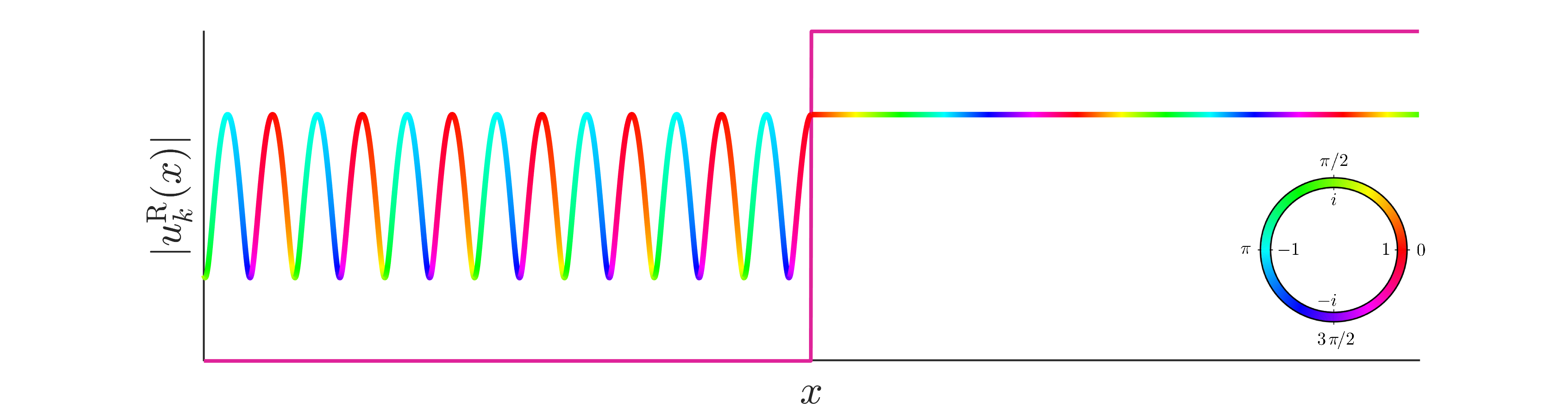— Figure 12.4:**Right-moving energy eigenstate**. Colour plot of a right-moving energy eigenstate, given in (12.14). For illustrative purposes, we also plot the potential step, to highlight where it is in relation to the wavefunction. On the left of the step, where there is both the incoming and reflected component of the wavefunction, there is interference, leading to sinusoidal oscillations. On the right, where there is only the transmitted component, the modulus of the wavefunction is constant.

However, note that we have the same issue arising here as we did for the free particle — the wavefunction $u^\mathrm{R}_k(x)$ is unnormalisable. Although this is again unpleasant, we just need to use these wavefunctions in the same way as we did for the free particle: we need to form wave packets out of the stationary states, i.e. to superpose stationary states with a range of energies, which is equivalent to a range of $k$ . In doing so we will be able to form normalised wavefunctions. We will return to this in the next subsection.

Before going there, we can still interpret more quantitatively the scattering at the potential, in terms of so-called reflection and transmission coefficients.

12.4Reflection and Transmission coefficients¶

We will now introduce a pair of coefficients, which tell us, roughly speaking, how likely a particle is to reflect off the potential step, or how likely it is to not reflect — i.e. to be transmitted. There are two ways in which this can be done, both of which lead to the same answer. Here we will present the simpler method, which is more heuristic. In Exercise 12.1 we show that the same answer is arrived at more formally by considering the probability current $j(x,t)$ .

Heuristically, even though the wavefunction $u_k^\mathrm{R}(x)$ is not normalisable, we nevertheless treat $A$ as proportional to the amplitude of the ‘incoming’ wavefunction — whereby the particle is moving to the right, and $B$ as proportional to the amplitude of the ‘reflected’ wavefunction. $B$ tells us the relative amplitude to be reflected, and hence we can define the reflection coefficient $R$ as the modulus square of the ratio between the reflected and incoming amplitudes,

\vph R = \frac{|B|^2}{|A|^2} = \frac{(k - k')^2}{(k+ k')^2}.

(12.15)

We define the transmission coefficient to be such that $R + T = 1$ , i.e. such that the particle is either reflected or transmitted with probability 1, hence

T = 1 - R = \frac{4k k'}{(k + k')^2}.

(12.16)

It turns out that the transmission coefficient is also equal to

T = \frac{k'|C|^2}{k|A|^2}.

(12.17)

The reflection and transmission coefficients are plotted as a function of $k$ in Figure 12.5.

$Reflection and transmission coefficients. Plot of reflection and transmission coefficients for the finite step, as given in and . Here k_0 = \sqrt{2MV_0}/\hbar is the minimum value of k we can consider, corresponding to E = V_0. We see that the particle is perfectly reflected in this case, and that the reflection coefficient is large only for k close to k_0. For large values of k, the particle is transmitted with almost unit probability.$

Figure 12.5:Reflection and transmission coefficients. Plot of reflection and transmission coefficients for the finite step, as given in (12.15) and (12.17). Here $k_0 = \sqrt{2MV_0}/\hbar$ is the minimum value of $k$ we can consider, corresponding to $E = V_0$ . We see that the particle is perfectly reflected in this case, and that the reflection coefficient is large only for $k$ close to $k_0$ . For large values of $k$ , the particle is transmitted with almost unit probability.

As we can see, only when the energy $E$ of the incoming particle is close to the height of the step $V_0$ , corresponding to $k = \sqrt{2ME}/\hbar$ being close to $k_0 = \sqrt{2MV_0}/\hbar$ is there significant amounts of reflection. When the energy is much larger, corresponding to $k$ being much larger than $k_0$ , then the particle is transmitted with probability quickly approaching 1.

That is, for the transmission, we divide the amplitude squared for the particle to be transmitted by the amplitude square of the incoming particle, corrected by a factor of $k'/k$ . This factor comes because the particle slows down as it crosses the barrier, causing the probability amplitude to grow. This factor precisely takes into account how much a probability amplitude increases or decreases because of a change of velocity, which is calculated using the probability current.

In Exercise 12.2 we analyse the behaviour of the reflection and transmission coefficients as we vary the physical parameters of the problem — the height of the barrier $V_0$ , the mass of the particle $m$ , and the energy of the particle $E$ .

Exercise 12.1 (Reflection and transmission coefficients from probability current)

In this exercise, we will show that we can also arrive at the expressions for the reflection and transmissions coefficients by considering the probability current $j(x,t_0)$ .

Consider the wavefunction associated to the incoming particle, $\Psi_\mathrm{inc}(x,t_0) = A e^{ikx}$ at time $t_0$ , where $k$ is a positive constant. Show that the probability current for this wavefunction is
$j_\mathrm{inc}(x,t_0) = \frac{\hbar k}{M} |A|^2.$
(12.18)
Using your calculation from part 1, explain why the currents for the reflected wavefunction $\Psi_\mathrm{refl}(x,t_0) = B e^{-ikx}$ and the transmitted wavefunction $\Psi_\mathrm{trans}(x,t_0) = C e^{ik'x}$ are

\begin{align*} j_\mathrm{refl}(x,t_0) &= -\frac{\hbar k}{M} |B|^2,& j_\mathrm{trans}(x,t_0) = \frac{\hbar k'}{M} |C|^2. \end{align*}

(12.19)

We will now define the reflection and transmission coefficients as proportion of the incoming current that is reflected and transmitted respectively. We thus define $R$ and $T$ to be
$\begin{align*} R &= \frac{|j_\mathrm{refl}(x,t_0)|}{j_\mathrm{inc}(x,t_0)},& T &= \frac{j_\mathrm{trans}(x,t_0)}{j_\mathrm{inc}(x,t_0)}, \end{align*}$
(12.20)
where we use $|j_\mathrm{refl}(x,t_0)|$ , since by the physics of the problem, this is a negative quantity. Substitute in the expressions from part 1 and part 2 to show that we recover the expressions (12.15) and (12.17) from the main text.

Lesson

This shows that the reflection and transmission coefficients can be defined in terms of the probability currents as well as how they were defined in the main text, and both lead to the same answer.

Exercise 12.2 (Dependence of reflection coefficient on physical parameters)

In this exercise, we will explore the dependence of the reflection coefficient $R$ on the physical parameters of the problem, namely on the mass of the particle $m$ , and the height of the step $V_0$ .

By substituting the definitions of $k$ and $k'$ , show that the reflection coefficient can alternatively be written as
$R = \frac{\vph \left(\sqrt{E} - \sqrt{E-V_0}\right)^2}{\left(\sqrt{E} + \sqrt{E-V_0}\right)^2}$
(12.21)
What does this tell us about how the reflection coefficient depends upon the mass of the particle?
What happens when (i) the potential step vanishes, $V_0 = 0$ ? (ii) The energy of the particle equals the height of the potential, $E = V_0$ ?
Do both of your answers to part 3 make sense physically?

12.5Dynamics of wavepackets¶

Video: Scattering III

The most interesting phenomenon that we can study in this context is the motion of a wavepacket as it crosses the potential step. Unfortunately, this problem is actually completely intractable analytically. Nevertheless, conceptually the situation is identical to our treatment of wavepackets when considering a free particle, as we will outline below. In order to actually study anything in this case we have to turn to numerics. We will see an example of this at the end of this section.

Starting with the conceptual side, we would like to specify a wavepacket $\Psi(x,0)$ at time $t = 0$ , which is again a complete specification of the state. As a concrete example, we could imagine a packet with centre at $x_0 \ll 0$ , far from the origin, with width $\Delta x \ll x_0$ , such that the particle is initially completely on the left-hand side of the step. We can then consider that the particle has positive average momentum $p_\mathrm{av} \gg 0$ , and uncertainty in momentum $\Delta p \ll p_\mathrm{av}$ , so that the momentum of the particle is positive. For example, we could consider a Gaussian wavepacket, as we did for the free particle. Such a packet fits within our general picture of a particle coming from the left and moving to the right.

Such a wavepacket can be expressed as a superposition of energy eigenstates, just like in any other situation. Crucially, given the way we have just set things up, this wavepacket will in fact be a superposition only of the right-moving energy eigenstates $u_k^\mathrm{R}(x)$ . Thus, at $t = 0$ the wavefunction $\Psi(x,0)$ can be written as

\Psi(x,0) = \frac{1}{\sqrt{2\pi}}\int_{k_0}^\infty c(k) u_k^\mathrm{R}(x) dk,

(12.22)

for some function $c(k)$ which determines the shape of the wavepacket. Note that the lower limit of integration is $k_0 = \sqrt{2MV_0}/\hbar$ , as we want the particle to have enough energy $E > V_0$ , i.e. enough energy to pass the potential step.

We can now once again write down the wavefunction of the particle at an arbitrary time $t$ . This is because once again (12.22) is a decomposition of the wavefunction at $t = 0$ into energy eigenstates. These are stationary states, whose time evolution is simple, and we know that the superposition principle tells us that the time evolution of a superposition is the superposition of the time evolution, namely

\Psi(x,t) = \frac{1}{\sqrt{2\pi}}\int_{k_0}^\infty c(k) e^{-i\hbar k^2t/2M} u_k^\mathrm{R}(x) dk,

(12.23)

Evaluating this integral will in general only be possible numerically, but in principle this is the solution, in complete analogy to any other situation we have studied.

Example 12.1 (Gaussian wavepacket)

As an example, we can again consider a Gaussian wavepacket. Therefore, let us take the function $c(k)$ closely related to that from Example 4.1,

c(k) = \left(\frac{2 a^2}{\pi}\right)^{1/4}e^{-a^2(k-k_\mathrm{av})^2}e^{ikx_0}.

(12.24)

The only differences compared to (5.11) are that we centre the Gaussian now at $k_\mathrm{av} = p_\mathrm{av}/\hbar$ , and the final factor of $e^{-ikx_0}$ , which has the effect of translating the spatial wavefunction so that the initial wavepacket is approximately

\Psi(x,0) = \left(\frac{1}{a\sqrt{2\pi}}\right)^{1/2} e^{-(x-x_0)^2/4a^2}e^{ik_\mathrm{av} x}

(12.25)

corresponding to a Gaussian with centre at $\langle x \rangle = x_0$ and average momentum $\langle p \rangle = \hbar k_\mathrm{av} = p_\mathrm{av}$ .

To find the evolution in time, we can numerically evaluate (12.23), for a range of times, restricting the range of integration to where the Gaussian $c(k)$ is non-zero, which is around the value of $k_0$ . In Figure 12.6 we plot an animation of the result, encompassing the wavepacket approaching the step, and being partially reflected by it. We see that the final state of the particle is a superposition of two wavepackets — a reflected wavepacket and a transmitted wavepacket.

$Scattering of a Gaussian wavepacket by a potential step. An animation of the scattering of a Gaussian wavepacket by a step potential. In the top plot, we show the wavefunction |\Psi(x,t)| using a colour plot. In the bottom plot, we show the associated probability density |\Psi(x,t)|^2. The potential step is also plotted, for illustrative purposes. The particle approaches the step from the left, with positive momentum, and energy larger than the potential height V_0. Nevertheless, the particle is partially reflected by the step, such that the final state of the particle is a superposition of a left-moving packet after the step, and a right-moving packet that has been reflected by the step.$

Figure 12.6:Scattering of a Gaussian wavepacket by a potential step. An animation of the scattering of a Gaussian wavepacket by a step potential. In the top plot, we show the wavefunction $|\Psi(x,t)|$ using a colour plot. In the bottom plot, we show the associated probability density $|\Psi(x,t)|^2$ . The potential step is also plotted, for illustrative purposes. The particle approaches the step from the left, with positive momentum, and energy larger than the potential height $V_0$ . Nevertheless, the particle is partially reflected by the step, such that the final state of the particle is a superposition of a left-moving packet after the step, and a right-moving packet that has been reflected by the step.

12.6Finite square well¶

Video: Scattering IV

Finally, we can return to the finite square well, and consider energy eigenstates with $E > V_0$ . Our procedure is identical to above: we need to first need to solve the time-independent Schrödinger equation in the 3 regions — to the left of the well, inside the well, and to the right of the well. We should then identify our two physically relevant situations: a right-moving and a left-moving particle. Mathematically, this will allow us to set one of our integrations constants to 0. Finally, we need to stitch together the solutions in the 3 regions, using the continuity of the wavefunction and its first derivative in order solve for all but one of the remaining integration constants, with the final one being the normalisation constant, as always.

Here we simply state the final answer, which is obtained after a rather long and intricate calculation, that is carried out in Problem Sheet - Week 12 as a final, challenging, exercise for the course. The right-moving energy eigenstate with incoming energy $E = \hbar^2 k^2/2M$ is

u^\mathrm{R}_k(x) = \begin{cases} Ae^{ik' x} + B e^{-ik' x} & \text{if } x < 0, \\ Ce^{ik x} + D e^{-ik x} & \text{if } 0 \leq x \leq a, \\ Fe^{ik' x} & \text{if } x > a, \\ \end{cases}

(12.26)

where $k' = \sqrt{2M(E-V_0)}/\hbar$ , $A$ is the normalisation constant, and

\begin{align*} B &= \frac{2i(k^2-k'^2)\sin ka}{(k+k')^2 e^{-ika} - (k-k')^2e^{ika}}A,\\ C &= \frac{2k'(k+k')e^{-ika}}{(k+k')^2 e^{-ika} - (k-k')^2e^{ika}}A, \\ D &= \frac{2k'(k-k')e^{ika}}{(k+k')^2 e^{-ika} - (k-k')^2e^{ika}}A,\\ F &= \frac{4kk'e^{-ik'a}}{(k+k')^2 e^{-ika} - (k-k')^2e^{ika}}A. \end{align*}

(12.27)

This wavefunction is depicted in Figure 12.7, for two different values of $k$ , the significance of which will become clear below.

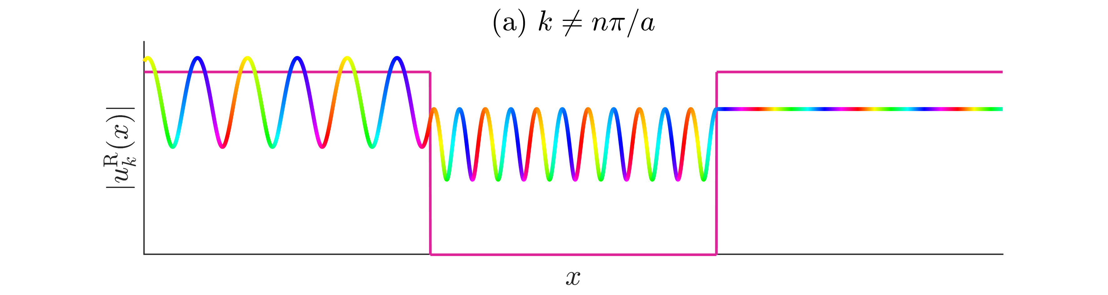
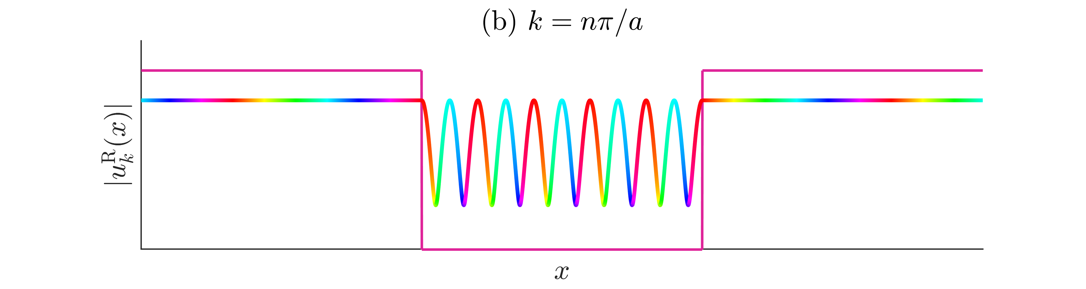
Right-moving energy eigenstates of the finite square well. Colour plot of a right-moving energy eigenstate, given in . For illustrative purposes, we also plot the potential step, to highlight where it is in relation to the wavefunction. (a) An example for a value of k \neq n\pi / a, for some integer a. The fact that the modulus varies to the left of the well and inside the well is an indication that in these regions the particle is moving both to the left and to the right. (b) An example for a value of k equal to a multiple of \pi/a. In these special cases, the particle is perfectly transmitted. As a consequence, to the left of the well the modulus is constant, signalling only a right-moving component of the wavefunction. — (a)

This wavefunction leads to the following reflection and transmission coefficients

\begin{align*} R &= \frac{(k^2-k'^2)^2 \sin^2 ka}{4k^2 k'^2 + (k^2-k'^2)^2 \sin^2 ka},\\ T &= \frac{4k^2 k'^2}{4k^2 k'^2 + (k^2-k'^2)^2 \sin^2 ka}. \end{align*}

(12.28)

As you can see, the solutions have a complex form, which is why they are being stated, and not derived. It it most interesting to look at the transmission coefficient graphically, which we plot in Figure 12.8.

Transmission coefficient of the finite well. Plot of transmission coefficient for the finite square well, as given in . Here k_0 = \sqrt{2MV_0}/\hbar is the minimum value of k we can consider, corresponding to E = V_0. We see that the particle is perfectly transmitted whenever k is a multiple of \pi/a, i.e. exactly the values of k which give the energy eigenstates of the infinite square well. Thus, if a particle has energy above E the height of the well V_0, but this energy happens to match the the energy levels of the infinite square well, it is not reflected at all by the potential well. — Figure 12.8:**Transmission coefficient of the finite well**. Plot of transmission coefficient for the finite square well, as given in (12.28). Here $k_0 = \sqrt{2MV_0}/\hbar$ is the minimum value of $k$ we can consider, corresponding to $E = V_0$ . We see that the particle is perfectly transmitted whenever $k$ is a multiple of $\pi/a$ , i.e. exactly the values of $k$ which give the energy eigenstates of the infinite square well. Thus, if a particle has energy above $E$ the height of the well $V_0$ , but this energy happens to match the the energy levels of the infinite square well, it is not reflected at all by the potential well.

What we see is that for certain values of $k$ the particle is transmitted with probability 1, while for other values this is not the case. The values of $k$ where $T$ becomes unity are those where $R = 0$ , which we see from (12.28) is when $\sin^2 ka = 0$ . This occurs when $k = n\pi/a$ . These are precisely the values of $k$ we found for the infinite square well!

Thus, if the particle has more energy then the well, i.e. $E>V_0$ , so that it is not bound in the well, and the energy happens to match one of the energy levels of the infinite square well, then the particle is not reflected at all, but is transmitted with unit probability. For any other value of $k$ , there is a probability that the particle is reflected. Thus, the quantisation condition of the infinite square well again appears for the finite well, now when considering scattering.

Finally, we can also consider the dynamics of wavepackets, just as we did in Section 12.5. Considering the same Gaussian wavepacket from Example 12.1, we plot the evolution in Figure 12.9.

Scattering of a Gaussian wavepacket by a potential well. A plot of the scattering of a Gaussian wavepacket by the finite square well. In the top animation we plot the wavefunction \Psi(x,t) using a colour plot. In the bottom animation, we plot the associated probability density |\Psi(x,t)|^2. The potential well is also plotted, for illustrative purposes. The particle approaches the well from the left, with positive momentum, and energy larger than well depth V_0. The particle is partially reflected by the left-hand wall, with part of the wavepacket entering, and part reflecting. The part which is transmitted then rapidly approaches the right-hand wall, where it is again partially reflected and partially transmitted. The part which is reflected then approaches the left-hand wall, where it can again be partially reflected and transmitted. At late times, the particle will be found outside the well, either travelling to the right or to the left, and with a spread-out form, accounting for the possibility of multiple reflections inside the well before finally escaping. — Figure 12.9:**Scattering of a Gaussian wavepacket by a potential well.** A plot of the scattering of a Gaussian wavepacket by the finite square well. In the top animation we plot the wavefunction $\Psi(x,t)$ using a colour plot. In the bottom animation, we plot the associated probability density $|\Psi(x,t)|^2$ . The potential well is also plotted, for illustrative purposes. The particle approaches the well from the left, with positive momentum, and energy larger than well depth $V_0$ . The particle is partially reflected by the left-hand wall, with part of the wavepacket entering, and part reflecting. The part which is transmitted then rapidly approaches the right-hand wall, where it is again partially reflected and partially transmitted. The part which is reflected then approaches the left-hand wall, where it can again be partially reflected and transmitted. At late times, the particle will be found outside the well, either travelling to the right or to the left, and with a spread-out form, accounting for the possibility of multiple reflections inside the well before finally escaping.

The new features we observe now compared to before, is that the particle will now repeatedly be transmitted and reflected by each wall of the well, leading to a much more intricate and complicated form at later times. Nevertheless, the general behaviour is as expected, even though we have the special energies which are perfectly transmitted by the well.