Chapter 11: The 3D infinite box

In this chapter we will apply what we learnt in the previous chapter to the mathematically simplest situation involving a particle confined in a three-dimensional potential well. The potential well we will consider is the direct generalisation of the infinite square well that we studied in Chapter 7: The infinite square well. We will refer to this as the 3D infinite box potential.

As we explained in Chapter 7: The infinite square well, the idea that a particle could have an infinite potential energy in some region isn’t particularly physical. Nevertheless, it provides us with a clean mathematical model which is easy to study, and it can be viewed as a fairly good approximation to a very deep potential well.

The main new ingredient we will encounter in this chapter is that in 3D energy levels become degenerate. This means that we will see that there are multiple different distinct energy eigenstates of the 3D infinite box, all with the same energy. While we have encountered energy degeneracy before in 1D, this only happened when the particle was non-bound. It is a new feature of 3D that we can have energy level degeneracy, and this is indeed a very important feature of nature (for example, the energy levels of Hydrogren are degenerate).

We will also see that even though we are now considering a 3D problem, what we learnt in 1D is still highly relevant. We will in particular see how the 1D energy eigenfunctions in fact compose to give us the 3D eigenfunctions. This is generically the case, and highlights the importance of studying 1D problems as a means for understanding the physics of more realisitic 3D problems.

11.1The 3D infinite box potential¶

We are going to consider a situation where a particle is perfectly confined inside a 3D ‘box’ — of volumne $L^3$ . That is, just like in 1D, that there are ‘walls’ at $x = 0$ and $x = L$ , as well as at $y = 0$ and $y = L$ and $z = 0$ and $z = L$ , leaving a perfectly cubic region in which the particle is confined. We can model this with the following potential energy function, the direct analogue of (7.1),

V(\rvec) = \begin{cases} 0 &\text{if }{0 \leq x,y,z \leq L} , \\ \infty &\text{otherwise,} \end{cases}

(11.1)

where $0 \leq x,y,z \leq L$ means that all three coordinates must individually be between 0 and $L$ . Unlike in 1D, it is no longer easy to depict this potential in a figure! Hopefully though it is straightforward to understand the basic geometry of this potential well.

Note that here we have chosen to take all 3 side lengths to be equal. This is a rather natural situation to consider, and will be the most interesting from the perspective of degeneracy. In Exercise 11.3 you will consider the most general situation, where all three side lengths differ.

11.2Energy eigenstates of the 3D infinite box potential¶

As always, our first goal in studying the 3D infinite box potential is to determine the energy eigenstates and associated energy eigenvalues. Since we have a particle confined inside a well, these will be bound states and so we expect that we will find discrete energy levels, just as we found in 1D.

As we spent some time arguing in 1D, due to the fact that the potential energy is infinite outside of the box, and given that physically we only want to consider that the particle has finite energy, it is natural to assume that the energy eigenfunctions will vanish outside of the box. That is, if we refer to the inside of the box as region I, and outside the box as region II, then we will look for energy eigenfunctions of the form

u_E(\rvec) = \begin{cases} u_E^{\rI}(\rvec) &\text{if }{0 \leq x,y,z \leq L} , \\ 0 &\text{otherwise,} \end{cases}

(11.2)

where $u_E^\rI(\rvec)$ is the function we would like to find. Since studying the infinite square well in Chapter 7, we subsequently saw in Chapter 8: The quantum harmonic oscillator that particles can tunnel into regions where they don’t have enough energy to be classically. We might therefore now be concerned about our assumption that the wavefunction vanishes outside the box. Although we don’t go further into this here, it can be shown that due to the infinite nature of the potential the wavefunction really does vanish outside of the box, and we are again in the exception circumstance where there is no tunnelling or barrier penetration.

We can therefore restrict our attention to the inside of the well. In this region, the Hamiltonian of the particle takes the simple form

\hat{H} = \frac{\hat{P}^2_x + \hat{P}^2_y + \hat{P}^2_z}{2M},

(11.3)

since inside the well the potential vanishes. The 3D TISE (10.35) therefore reads

\vph-\frac{\hbar^2}{2M}\left(\frac{\partial^2}{\partial x^2} + \frac{\partial^2}{\partial y^2} + \frac{\partial^2}{\partial z^2}\right)u_E^\rI(\rvec) = Eu_E^\rI(\rvec),

(11.4)

where the left-hand side is $\op{H}u_E^\rI(\rvec)$ .

Up until now we have only solved the TISE for a particle in 1D, which was then a partial differential equation in one variable. Now, for the first time, we need to study a partial differential equation in three variables, and understand how we can find its solutions.

Instead of approaching this head-on, we will try to analyse the structure a little, and in so doing, realise that we can spot the solutions.

In order to do so, let us first recall our solution to the 1D infinite square well. This was given in (7.14), namely,

u_n(x) = \begin{cases} \sqrt{\frac{2}{L}}\sin \frac{n\pi x}{L}&\text{if } 0 \leq x \leq L, \\ 0 &\text{if } x < 0 \text{ or } x > L. \end{cases}

(7.14)

The fact that these are energy eigenfunctions mean that inside the infinite square well (

0 \leq x \leq L

) they satisfy the relevant TISE, namely

-\frac{\hbar^2}{2M} \frac{\partial^2}{\partial x^2} \left(\sqrt{\frac{2}{L}} \sin \frac{n\pi x}{L}\right) = \frac{\hbar^2 n^2 \pi^2}{2ML^2} \sqrt{\frac{2}{L}} \sin \frac{n\pi x}{L}

(11.5)

from which we confirm that the corresponding energy eigenvalue is $E_n = \frac{\hbar^2 n^2 \pi^2}{2ML^2}$ .

Why is this relevant? Well, if we consider just the first term on the left-hand side of (11.5) — i.e. $\hat{P}^2_{x,\mathrm{w}}/2M$ — it is identical to the 1D TISE, except for the fact that in 1D the eigenfunctions were only a function of $x$ , while now we have a 3D function, of $\rvec$ . However, this isn’t a big problem, since if we consider any function of the form

u(\rvec) = u_n(x) f(y,z),

(11.6)

where $f(y,z)$ is some arbitrary function of $y$ and $z$ alone, then we see that we have essentially identical behaviour, and that, in fact, **any such function will be an eigenfunction of $\hat{P}^2_{x,\mathrm{w}}/2M$ . Namely,

\begin{align*} -\frac{\hbar^2}{2M} \frac{\partial^2}{\partial x^2} u(\rvec) &= -\frac{\hbar^2}{2M} \frac{\partial^2}{\partial x^2} \left(\sqrt{\frac{2}{L}} \sin \frac{n\pi x}{L}f(y,z)\right) \\ &= \frac{\hbar^2 n^2 \pi^2}{2ML^2} \sqrt{\frac{2}{L}} \sin \frac{n\pi x}{L}f(y,z),\\ &= E_n u(\rvec) f(y,z), \end{align*}

(11.7)

where we have used the fact that the partial derivative treats $f(y,z)$ essentially as a constant. The above confirms that $u(\rvec) = u_n(x) f(y,z)$ is an eigenfunction, with the eigenvalue $E_n$ as $u_n(x)$ .

Why has this helped us? Well, the next key step is to realise that we could make the same argument, but now focusing only on the $y$ component of the kinetic energy, $P^2_y/2M$ , or the $z$ component of the kinetic energy, $P^2_z/2M$ . In these two cases respectively, we would see that any functions of the form

\begin{align*} u'(\rvec) &= u_n(y)f'(x,z)& \text{and }&& u''(\rvec) &= f''(x,y)u_n(z), \end{align*}

(11.8)

would be eigenfunctions of $\hat{P}^2_{y,\mathrm{w}}/2M$ and $\hat{P}^2_{z,\mathrm{w}}/2M$ respectively, all with the same eigenvalue $E_n$ , for arbitrary functions $f'(x,z)$ and $f''(y,z)$ .

Now, we aren’t looking for eigenfunctions of an individual component of the kinetic energy. However, what we have seen above shows us that there is a way to find a joint eigenfunction of all 3 components! In particular, we see that if we find a function such that the behaviour in $x$ is $u_n(x)$ , the behaviour in $y$ is $u_n(y)$ and the behaviour in $z$ is $u_n(z)$ , then this will do the job! It is easy to write down such a function — it is just the product of the three individual functions! We only need to be careful and realise that we shouldn’t repeat $n$ 3 times, but consider 3 different values of $n$ , which we will call $n_x$ , $n_y$ and $n_z$ respectively. Thus, we arrive at the educated guess (also called ansatz frequently), that the energy eigenfunctions of the 3D box are of the form

\begin{align*} \vph u_\mathbf{n}(\rvec) &= u_{n_x}(x)u_{n_y}(y)u_{n_z}(z),\\ &= \begin{cases} \sqrt{\frac{8}{L^3}} \sin \frac{n_x \pi x}{L}\sin \frac{n_y \pi y}{L}\sin \frac{n_z \pi z}{L} &\text{ if } 0 \leq x,y,z \leq L, \\ 0 &\text{ otherwise,} \end{cases} \end{align*}

(11.9)

where, just as we did in 1D, we have changed notation from $u_E(\rvec)$ to $u_\mathbf{n}(\rvec)$ , labelling the energy eigenfunction by the vector of quantum numbers

\mathbf{n} = (n_x, n_y, n_z).

(11.10)

As an exercise you will confirm explicitly that these functions satisfy the TISE (11.4) with energy eigenvalue

E_\mathbf{n} = \frac{\hbar^2 \pi^2}{2ML^2} \left(n_x^2 + n_y^2 + n_z^2\right).

(11.11)

In what follows, it will be convenient to give a name to the combination $\frac{\hbar^2 \pi^2}{2ML^2}$ , which is a common multiple among all energy levels. We will denote this by

\Ebox = \frac{\hbar^2\pi^2}{2ML^2}.

(11.12)

Although we won’t prove it here, the energy eigenstates we have found in the above are in fact all energy eigenstates. That is, our educated guess in fact encompasses every energy level of the 3D infinite box, and doesn’t miss anything out.

11.3Degeneracy of the energy levels¶

Having obtained all of the energy levels of the 3D infinite box, we will now turn our attention to the one new property that arises in 3D which is new compared to 1D — degeneracy. It will be most instructive to start enumerating all of the energy levels and their corresponding energies. In order to

We do this in the following table:

Table 11.1:Energy levels of the 3D infinite box. We enumerate here the energy levels of the box, in increasing energy. As we can see, we have degeneracy: multiple distinct energy levels all with the same energy eigenvalue. Note: In the final column, we only write the form of the energy eigenfunction inside the box (and leave it implicit that outside the box the wavefunction vanishes).

$\mathbf{n} = (n_x,n_y,n_z)$	Energy $E_{\mathbf{n}}$	Energy eigenfunction $u_\mathbf{n}(\rvec)$
(1,1,1)	$3\Ebox$	$\sqrt{\frac{8}{L^3}} \sin \frac{\pi x}{L}\sin \frac{\pi y}{L}\sin \frac{\pi z}{L}$
(1,1,2)	$6\Ebox$	$\sqrt{\frac{8}{L^3}} \sin \frac{\pi x}{L}\sin \frac{\pi y}{L}\sin \frac{2\pi z}{L}$
(1,2,1)	$6\Ebox$	$\sqrt{\frac{8}{L^3}} \sin \frac{\pi x}{L}\sin \frac{2\pi y}{L}\sin \frac{\pi z}{L}$
(2,1,1)	$6\Ebox$	$\sqrt{\frac{8}{L^3}} \sin \frac{2\pi x}{L}\sin \frac{\pi y}{L}\sin \frac{\pi z}{L}$
(1,2,2)	$9\Ebox$	$\sqrt{\frac{8}{L^3}} \sin \frac{\pi x}{L}\sin \frac{2\pi y}{L}\sin \frac{2\pi z}{L}$
(2,1,2)	$9\Ebox$	$\sqrt{\frac{8}{L^3}} \sin \frac{2\pi x}{L}\sin \frac{\pi y}{L}\sin \frac{2\pi z}{L}$
(2,2,1)	$9\Ebox$	$\sqrt{\frac{8}{L^3}} \sin \frac{2\pi x}{L}\sin \frac{2\pi y}{L}\sin \frac{\pi z}{L}$
(1,1,3)	$11\Ebox$	$\sqrt{\frac{8}{L^3}} \sin \frac{\pi x}{L}\sin \frac{\pi y}{L}\sin \frac{3\pi z}{L}$
(1,3,1)	$11\Ebox$	$\sqrt{\frac{8}{L^3}} \sin \frac{\pi x}{L}\sin \frac{3\pi y}{L}\sin \frac{\pi z}{L}$
(3,1,1)	$11\Ebox$	$\sqrt{\frac{8}{L^3}} \sin \frac{3\pi x}{L}\sin \frac{\pi y}{L}\sin \frac{\pi z}{L}$
(2,2,2)	$12\Ebox$	$\sqrt{\frac{8}{L^3}} \sin \frac{2\pi x}{L}\sin \frac{2\pi y}{L}\sin \frac{2\pi z}{L}$
(1,2,3)	$14\Ebox$	$\sqrt{\frac{8}{L^3}} \sin \frac{\pi x}{L}\sin \frac{2\pi y}{L}\sin \frac{3\pi z}{L}$
(1,3,2)	$14\Ebox$	$\sqrt{\frac{8}{L^3}} \sin \frac{\pi x}{L}\sin \frac{3\pi y}{L}\sin \frac{2\pi z}{L}$
(2,1,3)	$14\Ebox$	$\sqrt{\frac{8}{L^3}} \sin \frac{2\pi x}{L}\sin \frac{\pi y}{L}\sin \frac{3\pi z}{L}$
(2,3,1)	$14\Ebox$	$\sqrt{\frac{8}{L^3}} \sin \frac{2\pi x}{L}\sin \frac{3\pi y}{L}\sin \frac{\pi z}{L}$
(3,1,2)	$14\Ebox$	$\sqrt{\frac{8}{L^3}} \sin \frac{3\pi x}{L}\sin \frac{\pi y}{L}\sin \frac{2\pi z}{L}$
(3,2,1)	$14\Ebox$	$\sqrt{\frac{8}{L^3}} \sin \frac{3\pi x}{L}\sin \frac{2\pi y}{L}\sin \frac{\pi z}{L}$

The reasons for including so many levels in this table is so that we can get a feeling for the complexity that arises. In particular, what we see is that the ground state is still a so-called non-degenerate energy level: there is a unique state of lowest energy (equal to $3\Ebox$ ), just like in 1D.

In contrast, the next two energies are both triply degenerate, at energy $6\Ebox$ and $9\Ebox$ . Where did this 3-fold degeneracy come from? If we look at the structure of $\mathbf{n}$ , we see it arises due to combinatorics: there are 3 vectors which have a single 2 and two 1s. With this insight, we see that any level of the form $\mathbf{n} = (n,n',n')$ (i.e. with a repetition in one of the quantum numbers) will be 3-fold degenerate, just as is the case for levels of energy $9\Ebox$ .

It is important to note that even though these states have the same energy, as you’ll confirm in an exercise, they are still nevertheless orthogonal states, e.g. $\inner{E_{(1,1,2)}}{E_{(1,2,1)}} = 0$ , because in the two cases the corresponding vector of quantum numbers is different.

The only other situation we can encounter is when $n_x \neq n_y \neq n_z$ . This happens for the first time when the energy is $14\Ebox$ . In this case, the combinatorics gives us 6 energy levels with the same energy, as there are 6 permutations of 3 numbers.

Finally, we also see that the level at energy $12\Ebox$ with $\mathbf{n} = (2,2,2)$ is non-degenerate, just like the ground state. This also follows from combinatorics: there is a single vector $\mathbf{n} = (n,n,n)$ for any integer $n$ (and no permutations).

All of the above degeneracies can be seen to arise due to symmetries — our ability to swap say $x$ and $y$ when $n_x$ and $n_y$ were equal. This didn’t actually change the energy eigenfunction, and this is why the energy has to be the same.

There is in fact another type of degeneracy that can arise, which isn’t due to symmetry, but is in fact just accidental. For example, the two levels $E_{(7,1,1)}$ and $E_{(5,5,1)}$ are degenerate, with energy $51\Ebox$ , because $5^2 + 5^2 + 1^2$ happens to be equal to $7^2 + 1^2 + 1^2$ . This has nothing to do with symmetry, and is just a particularity of the specific dependence of $E_\mathbf{n}$ on $\mathbf{n}$ (i.e. that it is the sum of the components squared).

In other potentials — such as Hydrogren — we will have a different degeneracy structure. It is important to realise however that it is precisely degeneracy that is the origin of the famous s, p and d shells that you may have already encountered, each being a different degenerate collection of energy levels.

11.4Evolution of particles inside a 3D box¶

As a final topic, we will now look at the evolution of a particle confined inside a 3D box. While on the one hand, the situation is just another example of what we have already encountered (i.e. an application of the superposition principle!), we will see that studying motion in 3D allows us to see more complex features, such as correlation between the different coordinates of the particle in time.

In the previous chapter, we already gave the general formulas for time evolution in 3D. Specicially, we saw that an initial state of the form

\ket{\psi_\init} = \sum_{\mathbf{n}} \alpha_{\mathbf{n}} \ket{E_\mathbf{n}},

(10.37)

evolves into

\ket{\psi(t)} = \sum_{\mathbf{n}} \alpha_\mathbf{n} e^{-iE_\mathbf{n} t/\hbar} \ket{E_\mathbf{n}}.

(10.38)

with corresponding wavefunction

\inner{\rvec}{\psi(t)}

\psi(\rvec,t) = \sum_{\mathbf{n}} \alpha_\mathbf{n} e^{-iE_\mathbf{n} t/\hbar} u_\mathbf{n}(\rvec),

(10.39)

Therefore, here we will consider a simple example, and see how we can analyse the behaviour. To that end, consider the specific initial wavefunction

\psi_\init(\rvec) = \frac{1}{\sqrt{2}}\left(u_{(1,1,1)}(\rvec) + u_{(2,2,1)}(\rvec)\right),

(11.13)

the wavefunction associated to an equal superposition of the ground state $\ket{E_{(1,1,1)}}$ of energy $E_{(1,1,1)} = 3\Ebox$ and the state $\ket{E_{(2,2,1)}}$ of energy $E_{(2,2,1)} = 9\Ebox$ , from the 3rd energy level. This state has $\alpha_{(1,1,1)} = \frac{1}{\sqrt{2}}$ , $\alpha_{(2,2,1)} = \frac{1}{\sqrt{2}}$ , and all other $\alpha_{\mathbf{n}} = 0$ .

Using the superposition principle, we can immediate write down the wavefunction of the particle at time $t$ , which is given by

\psi(\rvec,t) = \frac{1}{\sqrt{2}}\left(e^{-3i\Ebox t/\hbar}u_{(1,1,1)}(\rvec) + e^{-9i\Ebox t/\hbar} u_{(2,2,1)}(\rvec)\right).

(11.14)

We could stop here, but what is interesting is to analyse the properties of the particle. First, we can calculate the probability density $\pd(\rvec,t) = |\psi(\rvec,t)|^2$ . As you will confirm in an exercise, this is given by

\pd(\rvec,t) = \frac{1}{2}\left(|u_{(1,1,1)}(\rvec)|^2 + |u_{(2,2,1)}(\rvec)|^2 + 2\cos\frac{6\Ebox t}{\hbar} u_{(1,1,1)}(\rvec) u_{(2,2,1)}(\rvec)\right)

(11.15)

This is the probability density in 3D, but there is nothing to stop as asking questions about the probability density of any given coordinate. This is formally a marginal probability density, and we can obtain it by integrating out the coordinates we aren’t interested in (so that we get the total probability density for the remaining coordinate). For example, for the $x$ coordinate, we have

\pd(x,t) = \vph \infint \infint \pd(\rvec,t) dy dz.

(11.16)

In order to evaluate this, it will be advantageous to use the fact that the energy eigenfunctions of the 3D box are products of the eigenfunctions of the 1D infinite square well (as given in (11.9)). Focusing first on the first term on the right-hand side of (11.15), we see that

\begin{align*} \vph \infint \infint |u_{(1,1,1)}(\rvec)|^2 dy dz &= \infint \infint |u_1(x)|^2 |u_1(y)|^2 |u_1(z)|^2 dy dz, \\ &= |u_1(x)|^2 \infint |u_1(y)|^2 dy \infint |u_1(z)|^2 dz, \\ &= |u_1(x)|^2, \end{align*}

(11.17)

where in the first line we write the eigenfunction in terms of the eigenfunctions of the 1D infinite well, in the second line we have reorganised the integrals, and in the third line we have used the fact that the energy eigenfunctions of the 1D infinite square well are normalised, hence the integrals evaluate to unity (without having to do any work!).

We arrive at a similar conclusion for the second term on the right-hand side of (11.15), and see that after integrating over $y$ and $z$ , we are left with $|u_2(x)|^2$ . For the last term, the situation is interesting. The relevant integral is

\begin{align*} \vph \infint \infint u_{(1,1,1)}(\rvec)u_{(2,2,1)}(\rvec) dy dz & = u_1(x)u_2(x) \infint u_1(y)u_2(y) dy \infint u_1(z) u_1(z) dz, \\ &= 0. \end{align*}

(11.18)

Why is this zero? It is because of the integral over y. We should recall that the energy eigenfunctions of the infinite square are real. This means we could equally write $u_1(y)$ as $u_1^*(y)$ . The integral over $y$ is thus nothing but $\inner{E_1}{E_2}$ in disguise (as you have shown as an exercise in class, and where $\ket{E_1}$ and $\ket{E_2}$ refer to energy eigenstates of the 1D infinite square well). Since the energy levels are orthogonal (see (4.13)), the integral over y vanishes.

Putting everything together, we therefore see that

\pd(x,t) = \frac{1}{2}\left(|u_1(x)|^2 + |u_2(x)|^2\right),

(11.19)

which is independent of time! That is, if we only keep track of the x coordinate of the particle, this doesn’t change in time. Similar calculations, which you will do as an exercise show that similarly

\begin{align*} \pd(y,t) &= \frac{1}{2}\left(|u_1(y)|^2 + |u_2(y)|^2\right),\\ \pd(z,t) &= |u_1(z)|^2, \end{align*}

(11.20)

and are thus also independent of time.

What is this telling us? It actually shows that the motion in the different coordinates must be correlated, as the probability density $\pd(\rvec,t)$ is definitely not independent of time. It is actually the $x$ and $y$ coordinates that are correlated. We can study these by integrating over $z$ . As part of Exercise 11.5, you will show that

\begin{align*} \pd(x,y,t) &= \vph \infint \pd(\rvec, t) dz, \\ &= \frac{1}{2}\left(|u_1(x)|^2 |u_1(y)|^2 + |u_2(x)|^2 |u_2(y)|^2 + 2\cos\frac{6\Ebox t}{\hbar} u_1(x)u_2(x)u_1(y)u_2(y)\right) \end{align*}

(11.21)

In the following animation, you can see what this marginal probability density looks like:

Probability density in the x and y direction. An animation of probability density \pd(x,y,t) as given in . The z axis in this plot is \pd(x,y,t) (and not the box!). That is, we are ignoring motion along the z direction, just studying the motion of the particle in the x and y directions only. We see that the particle oscillates, between two distributions, each of which has two large peaks. If we look along only one direction, we can see how the individual probability densities \pd(x,t) and \pd(y,t) are time independent. 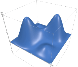— Figure 11.1:**Probability density in the $x$ and $y$ direction.** An animation of probability density $\pd(x,y,t)$ as given in (11.21). The $z$ axis in this plot is $\pd(x,y,t)$ (and **not** the box!). That is, we are ignoring motion along the $z$ direction, just studying the motion of the particle in the $x$ and $y$ directions only. We see that the particle oscillates, between two distributions, each of which has two large peaks. If we look along only **one** direction, we can see how the individual probability densities $\pd(x,t)$ and $\pd(y,t)$ are time independent.

As you can see, the particle oscillates back and forth, in a correlated fashion. In an exercise, you will study this correlation using the so-called covariance, a measure for how correlated the two coordinates of the particle are, on average at any given time. You will see that the coordinates oscillate between being correlated (both being large and positive / negative at the same time) to being anti-correlated (having opposite signs at a given time).

The main message here is that even simple superpositions of energy eigenstates can exhibit interesting correlated dynamics. This example is articifial, but hopefully from it you can see a glimplse of the rich dynamics that quantum particles exhibit in 3D.

11.5Exercises¶

Exercise 11.1

Confirm explicitly that the energy eigenfunctions of the 3D box potential

\begin{align*} \vph u_\mathbf{n}(\rvec) &= u_{n_x}(x)u_{n_y}(y)u_{n_z}(z),\\ &= \begin{cases} \sqrt{\frac{8}{L^3}} \sin \frac{n_x \pi x}{L}\sin \frac{n_y \pi y}{L}\sin \frac{n_z \pi z}{L} &\text{ if } 0 \leq x,y,z \leq L, \\ 0 &\text{ otherwise,} \end{cases} \end{align*}

(11.9)

satisfy the TISE (inside the box)

\vph-\frac{\hbar^2}{2M}\left(\frac{\partial^2}{\partial x^2} + \frac{\partial^2}{\partial y^2} + \frac{\partial^2}{\partial z^2}\right)u_E^\rI(\rvec) = Eu_E^\rI(\rvec),

(11.4)

and that the energy eigenvalues are given by

E_\mathbf{n} = \frac{\hbar^2 \pi^2}{2ML^2} \left(n_x^2 + n_y^2 + n_z^2\right).

(11.11)

Answer

n/a (show that)

Exercise 11.2

In this exercise we will confirm that two degenerate energy eigenstates are nevertheless orthogonal.

Write down the relationship between an energy eigenstate $\ket{E_\mathbf{n}}$ and the corresponding energy eigenfunction $u_\mathbf{n}(\rvec)$ .
Use part 1 to show that scalar product in terms of wavefunctions is given by

\inner{E_{\mathbf{n}}}{E_{\mathbf{n}'}} = \int_V u_{\mathbf{n}}^*(\rvec) u_{\mathbf{n}'}(\rvec) d^3\rvec.

(11.22)

Use the fact that $u_\mathbf{n}(\rvec) = u_{n_x}(x)u_{n_y}(y)u_{n_z}(z)$ (where $u_{n_x}(x)$ are the energy eigenfunctions of the 1D infinite square well, etc), and part 2 (along with its 1D analogue), to show that
$\inner{E_{\mathbf{n}}}{E_{\mathbf{n}'}} = \inner{E_{n_x}}{E_{n_x'}}\inner{E_{n_y}}{E_{n_y'}}\inner{E_{n_z}}{E_{n_z'}},$
(11.23)
where $\ket{E_{n_x}}$ is the energy eigenstate of the 1D infinite square well associated to $u_{n_x}(x)$ , etc.
Thus explain, using the orthogonality of the 1D eigenstates of the infinite square well, why energy eigenstates of the 3D box potential are orthogonal unless $\mathbf{n} = \mathbf{n}'$ (even if $\mathbf{n}$ and $\mathbf{n}'$ have component(s) in common).

Answers

$\ket{E_\mathbf{n}} = \int_V u_\mathbf{n}(\rvec) \ket{\rvec} d^3\rvec$ .
n/a (show that)
n/a (show that)
(11.23) shows that $\inner{E_{\mathbf{n}}}{E_{\mathbf{n}'}} \neq 0$ only if $n_x = n_x'$ , $n_y = n_y'$ and $n_z = n_z'$ simultaneously, i.e. $\mathbf{n} = \mathbf{n}'$ . Even if one or two components are same, remaining component in product will vanish.

Exercise 11.3

In this exercise we will consider an asymmetric box with walls at $x = 0$ and $x = L_x$ , $y = 0$ and $y = L_y$ and $z = 0$ and $z = L_z$ .

Write down the energy eigenfunctions and eigenvalues of a 1D infinite square well, with walls at $x = 0$ and $x = L_x$ .
Use part 1 to explain why a reasonable educated guess for the energy eigenfunctions of the asymmetric 3D box is
$\begin{align*} \vph u_\mathbf{n}(\rvec) &= &= \begin{cases} \sqrt{\frac{8}{L_x L_y L_z}} \sin \frac{n_x \pi x}{L_x}\sin \frac{n_y \pi y}{L_y}\sin \frac{n_z \pi z}{L_z} &\text{ if } 0 \leq x,y,z \leq L, \\ 0 &\text{ otherwise,} \end{cases} \end{align*}$
(11.24)
Confirm that (11.24) satisfies the TISE inside the asymmetric box, and determine the corresponding energy eigenvalues of the 3D box.
If $L_x = L$ , $L_y = \sqrt{2}L$ and $L_z = \sqrt{3}L$ , write down the first 5 lowest energy levels. Are there any degeneracies?

Answers

$u_n(x) = \sqrt{\frac{2}{L_x}}\sin \frac{n \pi x}{L_x}$ when $0 \leq x \leq L_x$ , and 0 otherwise; $E_n = \frac{\hbar^2 \pi^2 n^2}{2ML_x^2}$ .
This is the direct generalisation of the symmetric case from notes, with same product structure.
n/a (show that) for first part; $E_{\mathbf{n}} = \frac{\hbar^2 \pi^2}{2M}\left(\frac{n_x^2}{L_x^2} + \frac{n_y^2}{L_y^2} + \frac{n_z^2}{L_z^2}\right)$ .
In order: $E_{(1,1,1)}$ , $E_{(1,1,2)}$ , $E_{(1,2,1)}$ , $E_{(1,2,2)}$ , $E_{(1,1,3)}$ . No degeneracies.

Exercise 11.5

Starting from the wavefunction
$\psi(\rvec,t) = \frac{1}{\sqrt{2}}\left(e^{-3i\Ebox t/\hbar}u_{(1,1,1)}(\rvec) + e^{-9i\Ebox t/\hbar} u_{(2,2,1)}(\rvec)\right).$
(11.14)
show that the marginal probability density over $x$ and $y$ ,
$\pd(x,y,t) = \vph\infint \pd(\rvec,t) dz,$
(11.25)
is given by
$\pd(x,y,t) = \frac{1}{2}\left(|u_1(x)|^2 |u_1(y)|^2 + |u_2(x)|^2 |u_2(y)|^2 + 2\cos\frac{6\Ebox t}{\hbar} u_1(x)u_2(x)u_1(y)u_2(y)\right).$
(11.26)
Starting again from (11.14), show that the marginal probability density over $z$ ,
$\pd(z) = \vph \infint \infint \pd(\rvec) dx dy,$
(11.27)
is given by
$\pd(z) = |u_1(z)|^2.$
(11.28)
Write down an expression relating the marginal densities $\pd(y,t)$ and $\pd(x,y,t)$ .
Use part 3 to show that, starting from (11.26),
$\pd(y,t) = \frac{1}{2}\left(|u_1(y)|^2 + |u_2(y)|^2\right)$
(11.29)

Answers

n/a (show that).
n/a (show that).
$\pd(y,t) = \infint \pd(x,y,t) dx$ .
n/a (show that).

Exercise 11.6

In this exercise we will explore a measure of correlation known as the covariance. It is defined as

\mathrm{cov}(x,y) = \av{xy}-\av{x}\av{y},

(11.30)

where

\av{xy} = \vph \infint \infint xy \pd(x,y,t) dx dy.

(11.31)

The covariance is the difference between the expectation value of the product, and the product of the expectation values.

For the probability density
$\pd(x,t) = \frac{1}{2}\left(|u_1(x)|^2 + |u_2(x)|^2\right),$
(11.19)
making reference to Figure 7.5, explain why $\av{x} = \frac{L}{2}$ .

From (11.20), it is evident that $\pd(x,t)$ and $\pd(y,t)$ are identical in form, hence $\av{y} = \frac{L}{2}$ also.

Show that for
$\pd(x,y,t) = \frac{1}{2}\left(|u_1(x)|^2 |u_1(y)|^2 + |u_2(x)|^2 |u_2(y)|^2 + 2\cos\frac{6\Ebox t}{\hbar} u_1(x)u_2(x)u_1(y)u_2(y)\right).$
(11.26)
we have
$\av{xy} = \frac{L^2}{4} + \cos \frac{6\Ebox t}{\hbar} \infint x u_1(x) u_2(x) dx \infint y u_1(y) u_2(y) dy.$
(11.32)
Show that that
$\frac{2}{L}\int_0^Lx \sin \frac{\pi x}{L} \sin \frac{2 \pi x}{L} = - \frac{16L}{9\pi^2}.$
(11.33)
Hence calculate $\mathrm{cov}(x,y)$ (as a function of time).

Answers

$\pd(x)$ is the average of the prob. density of $u_1(x)$ and $u_2(x)$ . The average position of $\pd(x)$ is thus average position in ground state and first excited state. From figure, can see that prob. density is symmetric about centre of well for all eigenfunctions, so $\av{x} = \frac{L}{2}$ .
n/a (show that).
n/a (show that).
$\mathrm{cov}(x,y) = \left(\frac{16L}{9\pi^2}\right)^2 \cos \frac{6\Ebox t}{\hbar}$